Operations with sequences

In this section we will introduce the two main operations for sequences, namely addition (or subtraction) and multiplication by a scalar. For each of them we will explore how they affect the two properties we covered here, boundedness and monotonicity. We also briefly mention multiplication. These three operations work "term by term", which is a notion that will become clear in a second. At the end we introduce a different and less popular, yet important operation, convolution.

Addition (and subtraction) of sequences

Having two sequences {a_n} and {b_m}, we add them by forming a new sequence out of sums of individual terms of these two sequences. For this idea to work, the sequences have to be indexed in the same way. If one sequence's index starts earlier (for instance, if for {a_n} we have n = −1,0,1,2,3,... and for {b_m} we have m = 2,3,4,...), we can always start the "late" sequence a bit earlier by adding zeroes at its beginning, in this example we would put b₋₁ = 0, b₀ = 0, b₁ = 0, and now we can add them. However, this problem does not happen too often. In the following definition, we will for simplicity assume that the sequences are indexed in the same way and use the common index n for them.

Definition.
Consider sequences {a_n} and {b_n}. We define their sum as

{a_n} + {b_n} = {a_n + b_n}.

We define their difference as

{a_n} − {b_n} = {a_n − b_n}.

Using the long way of writing sequences (and assuming that the indexing is n = 1,2,3,...) we have

{a₁, a₂, a₃,...} + {b₁, b₂, b₃,...} = {a₁ + b₁, a₂ + b₂, a₃ + b₃,...}.

Similarly it works for subtraction.

It is easy to see that addition of sequences satisfies the laws of the usual addition. In particular, one has:
(1)     the commutative law: {a_n} + {b_n} = {b_n} + {a_n},
(2)     the associative law: ({a_n} + {b_n}) + {c_n} = {a_n} + ({b_n} + {c_n});
(3)     the zero element: {a_n} + {0}_n = {a_n},
(4)     the inverse element: {a_n} + {-a_n} = {0}_n.
Here {0}_n denotes the sequence {0, 0, 0, 0,...}, that is, a_n = 0 for all n.

How does addition influence the properties that we studied in Theory - Introduction - Basic properties? Some general statements can be made, we list just some of the more useful:

The sum of two bounded (in any sense) sequences yields a sequence bounded in the same sense.

The difference of two bounded sequences yields a bounded sequence.

Sum of a bounded sequence and an unbounded sequence (in any sense) yields a sequence unbounded in the same sense.

The difference of a bounded sequence and an unbounded sequence yields an unbounded sequence.

The first statement is quite simple. For instance, boundedness from below follows from the fact that if a_n > k and b_n > l for all n, then (a_n + b_n) > (k + l) for all n.

The second statement only works with boundedness, since if we subtract two sequences, both bounded from one side only, the same for both sequences, the resulting sequence might or might not be bounded in any sense. For instance,

{2, 0, 4, 0, 8, 0, 16, 0,...} − {0, 2, 0, 4, 0, 8, 0, 16,...} = {2, −2, 4, −4, 8, −8, 16, −16,...}.

Here we got a sequence not bounded in any sense. However, reasons for unboundedness might cancel by substraction:

{2, 4, 8, 16,...} − {2, 4, 8, 16,...} = {0, 0, 0, 0,...}.

Thus the second statement is basically the only possible in this direction.

You can surely think of some examples showing that while adding a bounded and unbounded sequence preserves unboundedness in any sense, mixing bounded and unbounded sequences by subtraction can lead to many different results.

Now what about these operations and monotonicity? We have the following.

The sum of two increasing sequences is an increasing sequence.
The sum of two decreasing sequences is a decreasing sequence.

We briefly sketch the proof of the first statement.

Denote {c_n} = {a_n} + {b_n}, so for every n we have c_n = a_n + b_n. Since we assume that both {a_n} and {b_n} are increasing, it follows that for every n we have a_n+1 > a_n and b_n+1 > b_n. For that particular n we can add these inequalities, obtaining a_n+1 + b_n+1 > a_n + b_n, which reads c_n+1 > c_n. Since we have shown that this inequality is true for all n, it follows that the sequence {c_n} is increasing as claimed.

Analogous statements work for non-increasing and non-decreasing sequences. When we add an increasing and a non-decreasing sequence, we get an increasing sequence. When we add a decreasing and a non-increasing sequence, we get a decreasing sequence. Proofs are similar to the one above.

When adding two monotone sequences of unknown type, we cannot say anything. For instance, when adding an increasing and a decreasing sequence, the tendencies of going up and going down start interacting and the stronger one wins. However, the size of steps up and down can differ throughout the sequence, so the resulting balance need not follow any monotonicity pattern. Consider the following example:

Example: Is
{1, 2, 5, 6, 9, 10, 13, 14, 17, 18, 21,...} + {5, 2, 1, −2, −3, −6, −7, −10, −11, −14, −15,...}
monotone?

Note that the first sequence is increasing and the second sequence is decreasing. The changes follow the same pattern; going from one term to the next, sequences always change first by one, then by three in the appropriate direction (up for the first, down for the second sequence).
However, adding them we obtain the sequence {6, 4, 6, 4, 6, 4, 6, 4, 6, 4, 6,...}, which is not monotone.

There are similar problems with subtraction, but general statements are still possible. For instance, if we subtract an increasing sequence from a decreasing one, we get a decreasing sequence.

Multiplication of a sequence by a scalar

Having a sequence {a_n}, we multiply it by a real number c by multiplying each term of the given sequence by c.

Definition.
Consider a sequence {a_n} and a real number c. We define their scalar multiple as

c{a_n} = {ca_n}.

Using the long way of writing sequences (and assuming the indexing is n=1,2,3,...) we have

c{a₁, a₂, a₃,...} = {ca₁, ca₂, ca₃,...}.

It is easy to see that scalar multiplication of sequences satisfies the laws we are used to from real numbers. In particular, one has:
(1)     the associative law: c(d{a_n}) = (cd){a_n};
(2)     the distributive law: c({a_n} + {b_n}) = c{a_n} + c{b_n};
(3)     the zero element: 0{a_n} = {0}_n.

Since this multiplication enlarges each term of a sequence by the same ratio, properties are basically preserved. First we dispose of a special case - the trivial case. If c = 0, then c{a_n} = {0}, so all the properties of the original sequence become irrelevant.
For a non-zero c everything depends on its sign. We have the following.

If c > 0, then c{a_n} has the same boundedness and monotonicity properties as the original sequence {a_n}.
If c < 0, then c{a_n} has boundedness and monotonicity properties of the original sequence {a_n} but always of the "opposite type".

For instance, if {a_n} is bounded from above, then -{a_n} = {-a_n} is bounded from below; if {a_n} is increasing, then -{a_n} = {-a_n} is decreasing.

Example:
Consider the sequence a_n = n² − 1 for n = 1,2,3,...; that is, the sequence {0, 3, 8, 15, 24,...}. This sequence is bounded from below but not bounded from above, it is also increasing.
The sequence (−2){n²−1} = {(−2)(n² − 1)} = {2 − 2n²}, written in the long way {0, −6, −16, −30, −48,...}, is then bounded from above but not bounded from below, and decreasing.

Multiplication of sequences

This is also done term-by-term. Since we work with two sequences here, we need them to be indexed in the same way.

Definition.
Consider sequences {a_n} and {b_n}. We define their product as

{a_n}⋅{b_n} = {a_nb_n}.

Using the long way of writing sequences (and assuming the indexing is n = 1,2,3,...) we have

{a₁, a₂, a₃,...}⋅{b₁, b₂, b₃,...} = {a₁b₁, a₂b₂, a₃b₃,...}.

This multiplication is not very useful, however, and is rarely used. It satisfies the laws of the usual multiplication of real numbers, including the distributive law; as the multiplicative unit one has the sequence {1}_n = {1, 1, 1,...}.

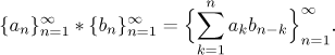
Convolution is an operation that in most applications of sequences replaces multiplication. It is taken with the same priority as multiplication in algebraic calculations; in particular, it has higher priority than addition of sequences. It is usually denoted by a star. Again, it requires that the sequences be indexed in the same way. We will assume here that the indexing starts at 1.

Definition.
Consider sequences {a_n} and {b_n}, where n = 1,2,3,... We define their convolution as

Written in the long way it is

{a₁, a₂, a₃,...} * {b₁, b₂, b₃,...} = {a₁b₁, a₁b₂ + a₂b₁, a₁b₃ + a₂b₂ + a₃b₁,...}.

This may look strange but in fact it is very useful in many applications. The idea is as follows: The first term of the convolution is one product, namely of the first terms of the given sequences. The second term is a sum of two products and so on. The term with index n (the n-th term) is a sum of n products, the first product is a₁b_n, then you start simultaneously increasing the index at a and decreasing the index at b by one until they reverse completely, that is, until you get to a_nb₁.
It is easy to see that one could also run the indexes the other way, start with a_nb₁ and end with a₁b_n.

How does the definition change if we start indexing the given sequences at a different number, say, N? The resulting sequence will also start its indexing with N and all the appearances of 1 in the definition of convolution will be replaced by N. Since in many applications, indexing n = 0,1,2,3... is required, we will show how convolution works then:

{a₀, a₁, a₂,...} * {b₀, b₁, b₂,...} = {a₀b₀, a₀b₁ + a₁b₀, a₀b₂ + a₁b₁ + a₂b₀,...}.

As you can see, the idea stays the same. It may be actually a bit easier if we call the resulting sequence {c_n} and show its terms:
c₀ = a₀b₀,
c₁ = a₀b₁ + a₁b₀,
c₂ = a₀b₂ + a₁b₁ + a₂b₀,...

The convolution satisfies the usual product rules. In particular, we have:
(1)     the commutative law: {a_n} * {b_n} = {b_n} * {a_n},
(2)     the associative law: ({a_n} * {b_n}) * {c_n} = {a_n} * ({b_n} * {c_n});
(3)     the unit element: {a_n} * {1, 0, 0, 0, 0,...}={a_n},
(4)     the distributive law: ({a_n} + {b_n}) * {c_n} = {a_n} * {c_n} + {b_n} * {c_n}.

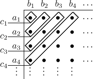
There is a handy matrix way of calculating convolution that some people like to use. To find {c_n} = {a_n} * {b_n}, start by listing the terms of {a_n} along the left edge and the terms of {b_n} along the top edge of an imaginary infinite matrix. Then we find all entries of this matrix by multiplying the corresponding row and column headers for each of them.

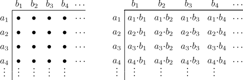
To find the terms c_n of the convolution, add the product along diagonals.

As an example we will calculate {1, −1, 2, −2, 3, −3,...} * {1, 2, 3, 4, 5, 6,...}:

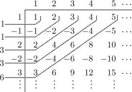
So

{1, −1, 2, −2, 3, −3,...} * {1, 2, 3, 4, 5, 6,...} = {1, 1, 3, 3, 6,...}

It is not obvious from this result how the convolution should go on, but it seems likely that terms of the outcome come in pairs. I tried a 10 by 10 matrix and came up with {1, 1, 3, 3, 6, 6, 10, 10, 15, 15,..}. The suspicion that numbers come in pairs is even stronger, but what numbers are these? What sequence goes 1, 3, 6, 10, 15,...? The answer can be guessed, since people who work with sequences will find these numbers familiar: Its n-th term is the sum 1 + 2 +...+ n. Thus after 15 the next number should be the sixth term of this sequence, that is, 1 + 2 + 3 + 4 + 5 + 6 = 21. Check it by calculating the next term in the convolution. Now we have a nice hypothesis, but proving it can be rather hard, so we leave it to experts.

The convolution is not really used when working with sequences as such, that is, when investigating their behaviour. We will therefore refer to various applications for further study of its properties. Here in Math Tutor convolution appears in two places, namely when we introduce multiplication of series and also multiplication of power series; there is plays a crucial role.

Back to Theory - Introduction