Split functions

Split functions (or functions defined by cases) actually appear quite often, in particular because the only reasonable way to investigate functions featuring absolute value is to get rid of the absolute value by splitting the expression into two cases (or more, if it features more absolute values). How do we work with such a function?

The basic rule is this: We analyze every expression that defines the given function on some set M in the usual way, but then we have to restrict the conclusions only to that set M. After we do this with all expressions and sets, we "put the resulting pictures side by side" to get the picture of the whole function. Again, there are two basic approaches. We can do the whole analysis of each expression separately and put the answers together at the end. The other approach is to combine information from all defining expressions at every step. We will now show both approaches. We will skip details, for more information about particular stages see appropriate sections in Methods Survey - Graphing.

Example: Sketch the graph of the function

f (x) = x³ + |x³| + 3x² - 9x - 3|x| - 45.

Solution: The domain is the whole real line, the function is continuous there. Before we go further we get rid of the absolute value.

As we wrote before, we now have two possible strategies.

1. Draw each formula separately.
This is actually something I rarely do, but in this example it is simple.

The first expression gives an upward-oriented parabola. We best identify its shape by finding roots and its vertex. For the roots we have the quadratic formula, we obtain x = −3 and x = 5. The vertex corresponds to the local minimum, which we found by solving f ′ = 0. We find that this local minimum is at the point (1,−48). So we can sketch the parabola, but in fact we will be only interested in the part above the negative half-axis, the endpoint is at f (0) = −45.

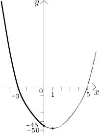
The second expression is a cubic curve. We identify it by finding roots and the two "bends". When we try to substitute some small integers, we soon guess that x = 3 is one root. We divide:

(2x³ + 3x² - 12x - 45) : (x - 3) = 2x² + 9x + 15.

This quadratic expression has no roots, so the cubic curve goes across the x-axis only at one point.

To find the "turns" we look for local extrema by solving f ′ = 0, we find out that there is a local maximum at (−2,−24) and a local minimum at (1,−52). To make the picture more precise we also find the inflection point (−1/2,−38−1/2) using the second derivative. Now we can sketch the cubic curve, but in fact we will be only interested in the part above the positive half-axis.

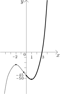
Now we put the pictures together and we get the graph of the function f. We should do one more thing to make the graph really good: We check on one-sided derivatives at 0. We get f ′₊(0) = −12 and f ′_-(0) = −6. This shows that at the connecting point we have a sharp bend, not a smooth connection.

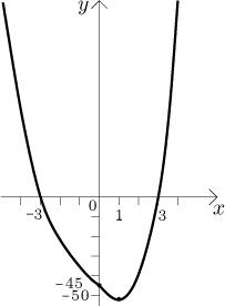
The important properties of f (monotonicity, concavity) can now be recovered from properties of the two curves using some common sense.

2. Step-by-step integration of data.
This approach calls for doing all steps simultaneously for all expressions involved in the definition of the function. At each step we right away ignore information that comes out of expressions but is not relevant to f, since it does not lie in regions where the expression in question agrees with f. It is a good idea to structure such a procedure to remind oneself that we always have to compare results to regions of validity. I usually divide real line into regions and create columns in which I work, in each column I only use the expression in its heading and cross out all conclusions that are outside this particular column.

To show this procedure we will return to the Example above. We actually did some steps easily using the original form with absolute value. To show the merging procedure in full generality we will ignore the given form and pretend that the function is given from the start by cases:

We start with the domain. Each expression exists on the set where it gives f and these sets combine to the whole real line, this is then the domain. The expressions for positive and negative halves do not look similar, so we suspect that this function is not symmetric. We confirm this suspicion when we try to substitute two symmetric points:

f (1) = −52,     f (−1) = −36.

Note that we crossed out the root 5, since it does not belong in the part of the real line where we work; in other words, at x = 5 the quadratic expression that lead to it has nothing to do with f.

Next we look for limits at endpoints of intervals in the domain and from the definition. For each area we again use appropriate formulas.

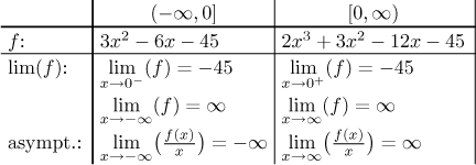
Since also f (0) = −45, the function is continuous at 0, at all other points its continuity follows from continuity of the defining expressions on appropriate intervals. We also see that there are no horizontal asymptotes at infinity and negative infinity, the last row rules out oblique asymptotes.

The next step is to find the derivative and determine monotonicity.

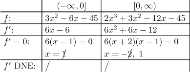
We have one critical point x = 1 and of course the dividing point x = 0 (where the derivative is suspect, so it actually also counts as a critical point), thus we have three intervals of monotonicity.

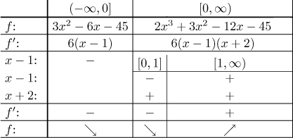
We put in the row with (x − 1) twice, once for the derivative on the left and once for the derivative on the right, because we wanted to make a point, namely that each factor of the derivative is evaluated (for sign) only in regions where the appropriate expression applies. In real life we would put it just once. Of course, in real life we would usually get distinct factors for each expression.

Back to the table. We see two adjacent intervals with the same monotonicity. Can we connect them? Since the function f is continuous at 0, we definitely can. Thus the conclusion is that f is decreasing on (−∞,1] and increasing on [1,∞). We have a local extreme, f (1) = −52 is a local minimum.

The last step is to find the second derivative and determine concavity.

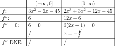
There are no separating points (apart from the default x = 0), so the original two intervals are intervals of concavity.

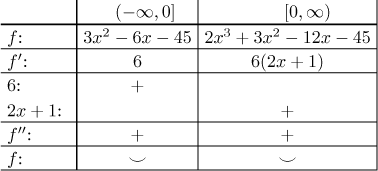
Thus f is concave up on (−∞,0] and on [0,∞).

The standard steps are done, here we also look at one-sided derivatives at 0 to get the connection right. We get f ′₊(0) = −12 and f ′_-(0) = −6. Then we put it all together.

First we choose the scale. Since we only have values between −3 and 3, we put the range between −5 and 5 (to have some elbow room) on the x-axis. Values we have here range from 0 (the x-intercepts) to −52. To squeeze it all in we decide to shrink the y-axis ten times compared to the x-axis.

Next we put in all points that showed up in all steps, namely f (−3) = 0, f (0) = −45, f (1) = −52, and f (3) = 0. Finally we combine the information on monotonicity and concavity to get the picture.

Some might find it helpful to actually merge the two tables before we draw the graph.

For other examples see this problem with a split function and this problem with absolute value in Solved Problems - Graphing.

Back to Theory - Graphing functions