Sketching parametric functions

Consider a parametric curve given by equations
x = x(t),
y = y(t)   for t in some interval I.
Assume that the functions x(t), y(t) are twice differentiable on I. We want to sketch this curve.

First we will try to see as much as possible with the description we have and then we will use the function approach. Most of it is common sense; the most important thing to keep in mind is that we will be mixing a "time" point of view and a spatial point of view, moving information from one framework to another. Knowing where you stand at any given phase of calculations is crucial and also pretty much sufficient for success. In order to illustrate out reasoning we will simultaneously work on an example.

Example: Investigate the parametric curve
x = (t − 1)²,
y = t³,   t ≥ 0.

Theory: What can we say from the description itself? The first important information is about the ends. If the interval I includes some of its endpoints, then substituting this time into x and y we learn where the path starts or ends. If some endpoint is not included, then we find the appropriate one-sided limit of x and y with respect to t. Interpreting this information can be interesting. If both limits are proper, then the curve simply goes toward the point we obtained. If both limits are improper, then the curve goes to one of the corners. Common sense should guide us, for instance if x→∞ and y→∞, then the curve goes toward the upper right corner; if x→−∞ and y→∞, then the curve goes toward the upper left corner. Then it is possible to ask about asymptote using appropriate modifications of the usual formulas. A line y = A⋅x + B is an asymptote if

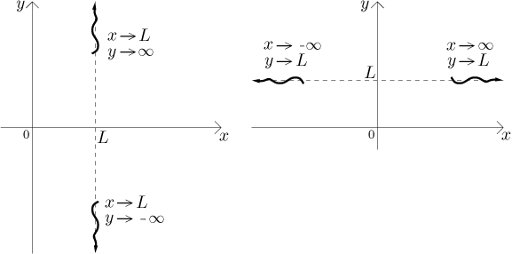
An interesting case is when one limit is proper and one improper. We then obtain a horizontal or a vertical asymptote as suggested in this picture:

Another traditional piece of data is intercepts. The x-intercepts are given by times t satisfying y(t) = 0, while the y-intercepts are given by times t satisfying x(t) = 0. We substitute each such time to both x and y and obtain points in the plane through which the path goes. By the way, when marking points, it is good to also mark at what times they were attained, since it helps in tracing the path.

Back to our Example: The interval I = [0,∞) contains its left endpoint, therefore we can substitute t = 0 into x and y and obtain the point (1,0). The other endpoint of I is infinity, so we find

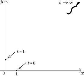
Thus the curve starts at the point (1,0), then goes around and eventually disappears in the upper right corner. Since y/x goes to infinity as time goes to infinity, it follows that there is no asymptote there (it also suggests that the curve turns more toward the y-infinity than toward the x-infinity; that is, it should curve upward in the picture).

Intercepts: The y-intercept is given by (t − 1)² = 0, which has just one solution, t = 1. This time gives the point (0,1). Now we look for x-intercepts. The equation t³ = 0 has only one solution t = 0, which gives the point (1,0).

Theory: Now we look for other points from the curve. Of course, we want "important" points, points where something changes. We start with x. This variable records movement in horizontal direction, so when x grows, the path moves left to right. If x decreases, the path moves right to left. Local extrema of x as a function are turning points for the path. Thus the next natural step is to investigate x itself as a function for monotonicity, but instead of increase/decrease we will interpret the signs of its derivative as right/left movement of the path. The times t that give local extrema of x will, when substituted into x and y, give turnaround points.

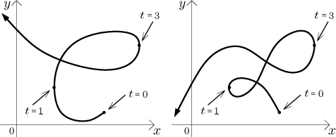
Note that this information is not enough to get a good sense of the path. In the following picture, both curves have identical turnaround points with respect to x and identical left/right directions, but they are rather different.

To get better information we similarly investigate the function y that gives vertical movement, so when we investigate it as an independent function, then the times t giving local extrema will show points where the path changes between going up and down.

Back to our Example: We find (t) = 2(t − 1), it has one critical point t = 1, so we get

The turnaround time t = 1 gives the point (0,1), we already had it as an intercept.

We also have (t) = 3t², it has one critical point t = 0, but that's the endpoint of I and no new intervals come out of it.

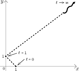
We get a better idea of the direction of the path when we combine the separate tendencies together.

Now we know the basic directions and we can sketch a rough picture.

Note an interesting thing. When we look at pieces of this curve as on graphs given by some y(x), then the direction in which we go along the path becomes irrelevant. Thus in the first part of the journey above, for times between 0 and 1, the bug or whatever goes upward, but the shape as a graph is decreasing. Indeed, the following picture shows that two different movements can lead to identical monotonicity of a graph.

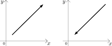
In the chart above this corresponds to disregarding the arrows, then we just get increasing or decreasing tendencies of a graph. Note that the picture above shows that we get an increasing graph for combinations + + and − − of signs of and . On the other hand, combinations of + − and − + give a decreasing graph. This should remind you of the sign algebra and it is no coincidence, since the spatial derivative of the function giving the graph is y′ = / (see the previous section). Thus indeed the sign of the spatial derivative is determined by the signs of individual derivatives of coordinates using the sign algebra.

So far we did not really need the function point of view. As we just saw, we can investigate the left-right and up-down movement, or we can consider a function y describing the graph and investigate its sign, in the end we get the same tendencies of the curve. However, now we would like to refine the picture, which calls for concavity and there we do need the function approach.

We recall the formula for the second spatial derivative:

Back to our Example: In our case we get

What are the dividing times for concavity? From the numerator we have t = 0 and t = 4/3, the denominator gives t = 1 (when the derivative does not exist). We get

The time t = 4/3 gives the point (1/9,64/27). This concludes the "standard" part. Here we do few more things. When drawing a graph that starts at a proper point, we usually also look for one-sided derivative there. Here

Now we should be able to sketch the curve. Since we have little information about times beyond 4/3, we try t = 2 and get the point (1,8). Since the curve goes up quite fast, it seems like a good idea to shrink the y-axis with respect to the x-axis to fit the picture in better.

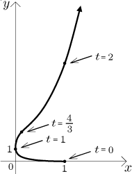
One more trick to try: When the time is really big, then x is approximately t². We can express t from this, substitute into y and we learn that for really large times the curve looks like the graph of y = x^3/2.

Back to Theory - Implicit and parametric functions