Area of a planar region

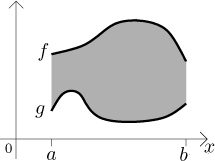
We know that the definite integral gives the mathematical area of the region between the graph of the integrated function and the x-axis. This will be our starting point for deriving some convenient formula for geometric area. First we choose the right object: a region between two graphs on the same interval.

Such a region is the best possible. First, it is general enough, second, it can be handled easily. Note that in our picture, both functions are positive, hence their definite integrals will give the geometric areas of regions under their graphs. The region between them can be easily obtained by subtracting the area under g from the area under f:

This formula turns out to be the right one for the general setting, we just have to be careful to identify the larger function. To see why this is true, consider now an example where the functions do not stay positive:

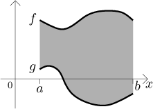
We split the region into vertical strips of width dx. Just like when we talked about the meaning of the definite integral, we may assume that the strips are so thin that the corresponding pieces of graph are straight lines.

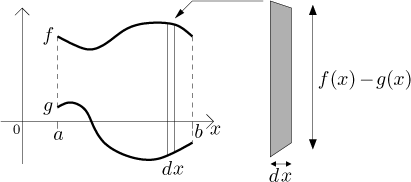
The area of one such strip is equal to the base dx multiplied by the height in the middle, which is f (x) − g(x), here we use the fact that f is the larger function. Thus

In any case, we get the following:

Fact.
Consider the region bounded from above by the graph of a function f and from below by the graph of a function g on an interval [a,b]. If the two functions are Riemann integrable, the area of this region is

It is possible to put the difference of functions into an absolute value, then we do not have to worry which of them is larger. Such a formula would be more general and elegant and therefore preferable from the mathematical point of view. However, since we do not know how to integrate absolute value directly, in concrete calculations we would end up splitting the integral into pieces depending on which function is larger at what place anyway.

Note: It is not helpful to split the area into horizontal strips (of size dy).

As you see in the picture, we end up with strips of different kinds. Some strips start at the level of x = a and go all the way to the level of x = b, while others start or end earlier, when they reach the graph of f or g. Close to the lower end we even have the situation when to a given level y we do not get one horizontal strip, but several strips one after another.

This means that we cannot find one common formula describing their lengths, which means that there is no way to create a general formula for adding their areas together, that is, there is no formula for the area of the whole region as a sum of horizontal strips. In fact, even the situation in the above picture is too nice. In general the graphs of f and g might oscillate up and down a lot and the situation becomes unmanageable.

Clearly there is no way to find the area like this using horizontal stripes, but vertical strips will work nicely.

Consider a parametric curve x = x(t), y = y(t) for t from [α,β]. Assume that y(t) ≥ 0 for all t and x(t) is increasing:

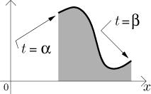
We can apply the splitting trick as above to the region under this curve. What is the area of one vertical strip? The height (in the middle) of such a strip is given by y(t). The width is given by dx, but the variable x is a transformation of variable t, for which we have a formula (see Theory - Integration - Substitution): dx = x′(t)dt. Thus we get

It is also possible to use the parametric equations to eliminate the parameter t using the inverse function to x, thus moving to the graph of a function setting. Note that we were using the symbol x for two objects: the variable and the function that specifies how the variable x depends on t. So far we could handle it, but in the following calculation it would get too confusing. We therefore decide for the moment to call this function by h, so now x = h(t). Now we are ready to identify the function f that gives the same curve as described by the given parametric equations, using parameter elimination:

Now we find the area using indirect substitution:

If x(t) is decreasing, the curve goes "from the right to the left" and the derivative is negative. This is easily fixed using absolute value. We still need to make sure that the resulting integral exists, so we use continuity as the easiest way out and get the following:

Fact.
Consider a parametric curve x = x(t), y = y(t) for t from [α,β]. If y(t) ≥ 0 for all t, x(t) is monotone, and both x′ and y are continuous, then the area under this curve is

Area given by a curve in polar coordinates

Consider a curve in polar coordinates given by ϱ = ϱ(φ) for φ from [α,β]. Assume that ϱ(φ) ≥ 0 for all φ.

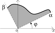
This time the shape of the region is different, so it is not possible to transform this situation into the above setting. We have to try it differently. Here we use the fact that the variable φ has a precise meaning - it is the angle. We therefore split the whole angle [α,β] into small sub-angles of size dφ, thus obtaining lots of "fans". Since they are so thin, we may assume that the outer side is not some curve but a piece of a circle centered at the origin.

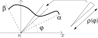
We know that the area of such a fan is given by half of the angle at the vertex in radians times its radius squared. Summing them up we get

We also have to make sure that the curve does not turn around more than once, because then the region would overlap and some area would be counted more times.

Fact.
Consider a curve in polar coordinates given by ϱ = ϱ(φ) for φ from [α,β], where β − α ≤ 2π. Assume that the function ϱ(φ) is continuous and that ϱ(φ) ≥ 0 for all φ. Then the area of the shaded region is

Curve length
Back to Theory - Applications