
Problem: Sketch the graph of the function

Solution: We will use the procedure as outlined in Overview of graphing in Methods Survey - Graphing. This is a genuine split function, so we have to treat it a bit differently than standard problems.
Step 1. The domain of a function defined by cases is the union of the sets from its description - that is, assuming that it was defined carefully and the expressions used in its definition really do exist on the sets where they are used. Since one can never be sure, we quickly check that every expression really does exist on the appropriate set. Thus the domain is
The defining expressions are all continuous wherever they are used, so we know that f is continuous on all intervals from its definition when considered open. However, it is not clear whether we can connect these intervals into larger intervals of continuity. We will return to this in Step 2.
Concerning symmetry, there is none, since the domain is not a symmetric set.
The x-intercept: We put all three expressions equal to zero. The
first equation we obtain cannot be solved algebraically, but fortunately we
are only interested in negative x and we notice that
Step 2. We find limits at endpoints of the intervals from the definition.
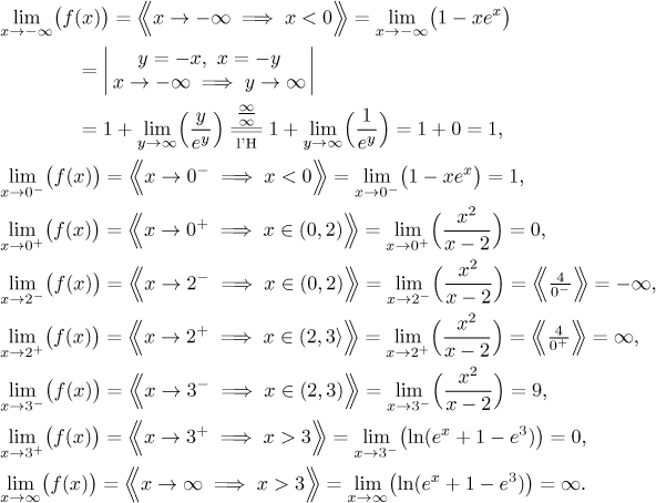
Now we are ready to talk continuity. We will make a chart summarizing situation at all connecting points.

We see that the limit at 0 and at 3 does not exist, so the function cannot be continuous there and the discontinuities there are not removable. On the other hand, all appropriate one-sided limits converge, so there are jump discontinuities at 0 and at 3. We also see that the function is continuous from the right at 0 and continuous from the right at 3. Because of the two discontinuities we cannot connect intervals from the definition to larger intervals of continuity; the best we can say is that f is continuous on every interval that appears in its definition.
Asymptotes: The candidates for
vertical asymptotes are proper endpoints of intervals from the domain and
points of discontinuity, thus the candidates are 0, 2, and 3. Both one-sided
limits at 0 converge, so there is not a vertical asymptote there. Similarly
we conclude that there is not a vertical asymptote at 3. However, at 2 we have
an improper one-sided limit (even both, but one is enough), so there is a
vertical asymptote at
The limit at negative infinity converges, so there is a horizontal asymptote
there, namely the line
Finally, the limit at infinity is infinity, so there is no horizontal asymptote there, but there is a chance for an oblique one. We apply the appropriate algorithm.
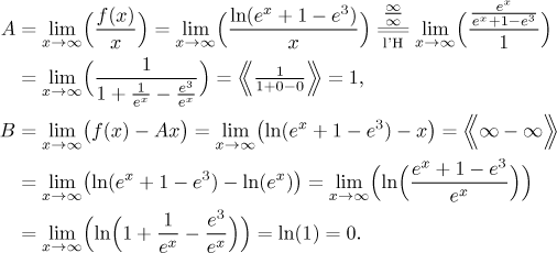
Since both limits converged, we have an oblique asymptote at infinity, it is
the line
Step 3. We find the derivative and use it to determine monotonicity and local extrema. Recall that derivative by rules only works on open intervals.
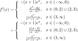
Critical points: Since the function is not continuous at 0 and at 3, it also does not have any derivative there and we have the first two critical points. Other points can be found by making the derivative equal to zero.
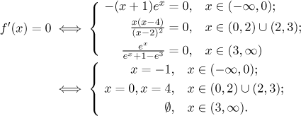
We have to disregard solutions that do not lie in regions where the particular formula agrees with f ′, which rules out 0 and 4. Thus we have critical points −1, 0, and 3, which splits the two intervals of domain into five intervals of monotonicity, we determine it using a table; we put closed endpoints when the function is continuous. As usual with split functions, we have to be careful where we apply various expressions.

We have adjacent intervals of equal monotonicity. Since there is a hole at 2 in the domain, we cannot connect there. However, there is a chance to connect intervals at 0. We could do it automatically if f were continuous there, but unfortunately this is not true. Thus we have to apply some common sense (see Monotonicity in Functions - Theory - Real functions). We know that f is decreasing on the left and on the right from 0, we also know that
f (0-) > f (0) = f (0+),
from which we conclude that we can in fact connect intervals of monotonicity at
0 (see the sketch below). The conclusion is that f is increasing on
Local extrema: The given function has a local maximum
By the way, if we put together information on monotonicity with limits at
endpoints above, we see that there is no
Step 4. We find the second derivative and use it to determine concavity. As in Step 3, we work in each region separately.

Dividing points: The second derivative does not exist at 0 and at 3 and it is zero at −2. These three points will divide the two intervals of the domain into five intervals of concavity, we determine it using a table; we put closed endpoints when the function is continuous.

The conclusion is that f is concave up on
Inflection point:
Step 5. Now we put it all together. First we put all points and limit
trends that we obtained above into a picture. This will be the skeleton on
which we will hang the function. In order to make the picture a bit smaller
we will not use the same scale on the
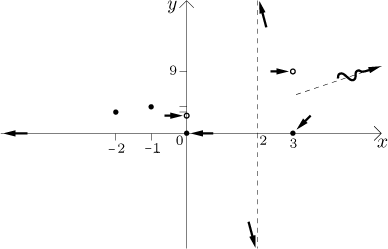
To see the shape of the graph better we combine the two tables above.

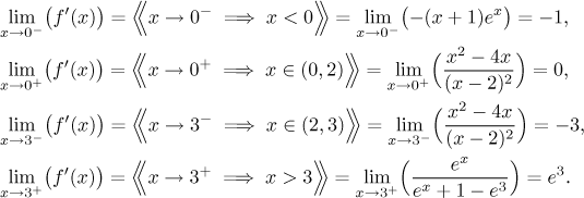
To make the picture more faithful we find limits of derivatives at points of discontinuity, so that we know in which directions the individual pieces of the graph should start off.
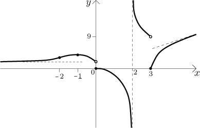
Now we are ready to sketch the graph.
Remark: When working with functions given by cases, we split the real line into several regions according to its definition and then do the algorithm several times, in each region, and in each of them we disregard results that are outside that particular region. The above calculations can be (briefly) expressed like this.
