Overview of graphing: Survey of methods

Assume that a function f is reasonable, which here means that its domain consists of at most countably many intervals, on each of which the function is twice differentiable. To sketch the graph of such a function we follow this procedure.

Graph sketching algorithm:
Step 1. Determine the domain of f, intercepts with axes (if possible), symmetry and periodicity, and continuity (sometimes with help from limits from Step 2). For more on these topics see Functions - Methods Survey - Real functions.
Step 2. Find appropriate one-sided limits at all endpoints of intervals from the domain of f, possibly also for individual intervals from the definition of f. For more info on limits see Functions - Methods Survey - Limits. Where appropriate, interpret these results as asymptotes, if necessary do the algorithm for oblique asymptotes, see Methods Survey - Graphing - Asymptotes.
Step 3. Find the derivative f ′. Use it to determine intervals of monotonicity and local extrema, for more details see Methods Survey - Graphing - Monotonicity and local extrema.
Step 4. Find the second derivative f ′′. Use it to determine intervals of concavity and inflection points, for more details see Methods Survey - Graphing - Concavity and inflection points.
Step 5. Draw the graph. Two strategies.
1) At each step of this procedure, put the acquired data into the picture, use it to make the picture more precise at each step.
2) First do all calculations, then put all points into the picture, then combine the information on monotonicity and concavity and create the final shape. For more details see Ingredients of graph sketching in Theory - Graphing functions.

Example: Sketch the graph of

Solution: D( f ) = (−∞,−1) ∪ (−1,∞), the function is continuous. Since the domain is not a symmetric set, the function cannot be symmetric either, it is not periodic.

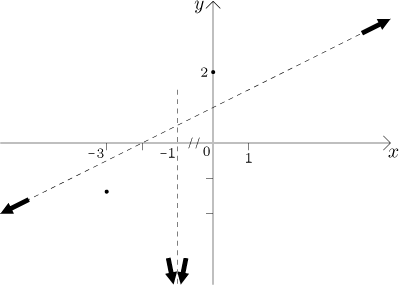
Intercepts: f (0) = 2, the equation  f (x) = 0 cannot be easily solved so we give up.

Limits at endpoints:

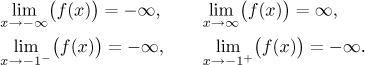
We see that there is a vertical asymptote at x = −1, using the appropriate algorithm we show that there is the asymptote y = x/2 + 1 at infinity and also at negative infinity (for details see Example in Methods Survey - Graphing - Asymptotes). By the way, since f goes to negative numbers at −1 and f (0) > 0, it follows that there must be an x-intercept between −1 and 0.

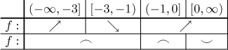
We find the derivative and use it to determine that f is increasing on (−∞,−3] and on (−1,∞), it is decreasing on [−3,−1). It has a local maximum f (−3) = −11/8 and a horizontal tangent line at f (0) = 2 (for details see Example in Methods Survey - Graphing - Monotonicity and local extrema).

We find the second derivative and use it to determine that f is concave down on (−∞,−1) and on (−1,0], it is concave up on [0,∞). It has a point of inflection f (0) = 2 (for details see Example in Methods Survey - Graphing - Concavity and inflection points).

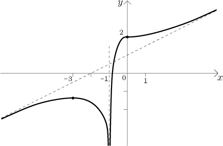
Calculations are done, it is time to sketch the graph. We draw coordinate axes and mark all points and limits at endpoints to anchor the graph.

Next we combine the charts of monotonicity and concavity to have a better idea of the shape of the graph.

Finally we "hang" this shape on the anchoring points in the picture to get the graph, we also use the info about a horizontal tangent line at 0.

Remarks:
If the function we are sketching has a proper one-sided limit at some proper endpoint (see Step 2), we need to know in which direction we should start drawing the graph from that point. This we find out by calculating the appropriate one-sided derivative at that point, most likely using a limit, and we need not worry about continuity in this particular case, see this note.

2. If f is a split function, then the best strategy is to do every step simultaneously for all expressions that define this function and collate the information. For more details see the section Split functions in Theory - Graphing functions, see also this example in Solved Problems - Graphing.

3. If f contains an absolute value (or more of them), then one should start by getting rid of them, writing the given function as a split function. See the appropriate example in Solved Problems - Graphing.

For other examples see Introduction in Theory - Graphing and appropriate problems in Solved Problems.

Monotonicity and local extrema
Back to Methods Survey - Graphing functions